Excel VLOOKUP Formula
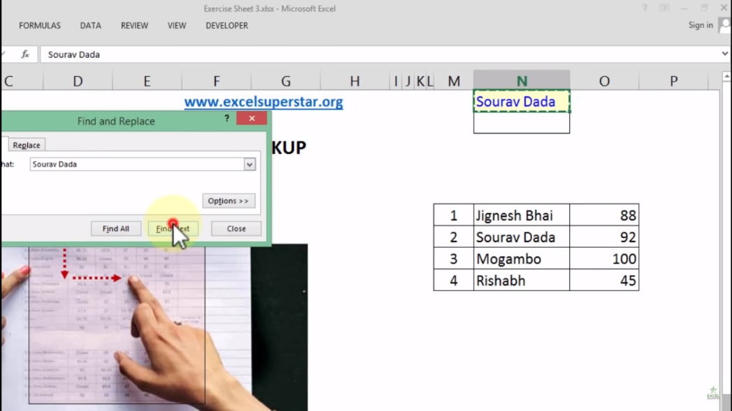


BONUS TIP
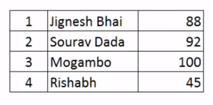
In this table I have added second column of Subjects. Now I want to find out the test scores scored by students in the second subject


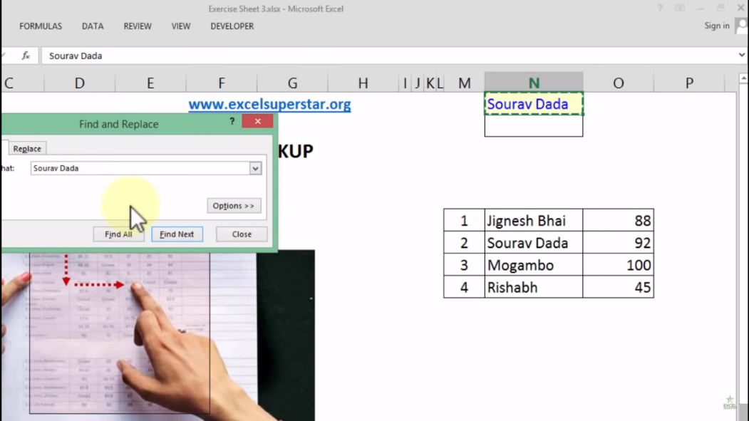
BONUS TIP
In this table I have added second column of Subjects. Now I want to find out the test scores scored by students in the second subject